Standard Deviation Calculator
Instant sample & population stats with step-by-step math
Show Step-by-Step Calculation & Deviation Table Expand
| # | Value (xᵢ) | Deviation (xᵢ − x̄) | Squared (xᵢ − x̄)² |
|---|
A visual spread chart often exposes patterns that polished statistical summaries conceal. When measurements fluctuate, population variability deserves careful attention, but a wider range alone does not prove the underlying process has become less reliable.
Before trusting any calculated result, check comma-separated values for missing entries or accidental duplicates. A step-by-step formula breakdown that shows the work makes subsequent calculations easier to audit, explain, and reproduce during routine technical reviews.
Table of Contents
What Is Standard Deviation?
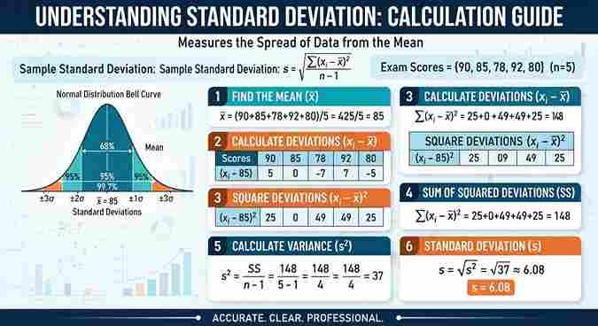
Two classes can share an identical mean yet differ sharply in spread. Standard deviation quantifies that dispersion across a dataset, using the square root of variance to express differences in the same units for comparisons.
A class teacher inspecting exam scores sees a low standard deviation when results cluster closely. A financial analyst tracks stock price volatility; a manufacturing engineer checks whether a production process remains consistent during routine inspections.
Standard Deviation Formula
An overlooked denominator can substantially change the result: a complete population uses N, while a sample uses n−1. This Bessel’s correction adjusts variance estimates because the observed mean already reflects the sampled data point values.
For population standard deviation, σ² = Σ(xᵢ − μ)² / N, then √σ². For standard deviation of a sample, s² = Σ(xᵢ − x̄)² / n−1, then √s². Two formulas quantify spread through squared differences.
Population Standard Deviation
With 5 observed values (1, 3, 4, 7, 8), the population mean μ is 4.6 through ∑x / N. Their population standard deviation σ reaches 2.577; unlike samples, the entire population needs N, not n.
Using summation notation, starting index i=1 identifies each individual value xi. The equation squares (xi − μ)²: 12.96, 2.56, 0.36, 5.76, 11.56. This summation yields variance after division by N; its square root defines σ.
Sample Standard Deviation
A random sample can look unusually consistent, so its sample standard deviation needs careful interpretation. Using the sample mean and n−1 adjusts the variance estimate for information lost when estimating the center from actual observations.
In practice, I check sample size before trusting s: small sample sizes produce unstable estimates across repeated studies. The equation uses Σ(xᵢ − x̄)² and degrees of freedom, while σ describes the unknown population spread.
Also Read: Cursive Font Copy Paste – Cursive Font GeneratorHow To Calculate Standard Deviation
Checking the sum prevents mistakes. This dataset contains 2, 3, 4, 4, 4, 5, 6, 6, 8, 10; its count is 10 and mean 5.2. Subtract x̄ from 4 to obtain −1.2; squaring gives 1.44.
The sum of squared deviations is 51.6. Divide by N: variance 5.16; its square root gives population standard deviation σ ≈ 2.271. Using n−1 gives sample standard deviation s ≈ 2.394, in the same units.
Worked Example: Test Scores {72, 85, 90, 68, 77}
Across 5 exam scores (72, 85, 90, 68, 77), total 392 yields an average exam score of 78.4. Deviation values are −6.4, 6.6, 11.6, −10.4, −1.4; their sum of deviations is 0, validating the mean.
Interpretation: 87 lies roughly 1 standard deviation above the mean. Squares: 40.96, 43.56, 134.56, 108.16, 1.96; total 329.20. Dividing by 4 gives sample variance (s²) 82.30 and sample standard deviation (s) 9.072, around 9 points.
Example 1: Calculate Sample Standard Deviation
The sample of 6 data values 30, 20, 28, 24, 11, and 17 produce a mean of 21.67. I retain extra decimals in the calculator before evaluating xi − x̄ and the square of differences.
Deviations 8.33, −1.67, 6.33, 2.33, −10.67, and −4.67 give a sum of squared differences near 253.33. Dividing by N−1 yields variance 50.67; the square root is 7.118, not 7.1169, when calculated using (xi − x̄)².
Example 2: Calculate Population Standard Deviation
Despite the high value of 27, σ equals 5.774 across this population: N = 6 data values, namely 10, 12, 18, 14, 21, 27. Their expected value µ is 17, rather than the range midpoint.
Audit xi − µ first: deviations −7, −5, 1, −3, 4, and 10 yield (xi − µ)² results 49, 25, 1, 9, 16, and 100. Their sum, 200, gives variance 33.333; take the square root.
Applications of Standard Deviation
In quality control, a core operational metric flags inconsistent products across industrial settings. With weather, a coastal city may show narrower temperature ranges than an inland city, partly because water has greater heat capacity naturally.
In finance, stock A and stock B can share a 10% average return despite different price fluctuations. Examining each asset distribution reveals risk, potential loss, and uncertainty before selecting a safer option for investment decisions.
Finance: Asset Volatility and the Sharpe Ratio
Matching stock returns can conceal different investment risk: annualized σ of 5% indicates low-risk fluctuations beside 40% high-risk exposure. I assess asset volatility under stressed trading conditions because volatility alone overlooks liquidity and potential losses.
Nobel laureate William F. Sharpe formulated the Sharpe ratio: S = (Rₚ − R𝑓) / σₚ. Excess return over portfolio standard deviation measures risk-adjusted performance; a higher Sharpe ratio reflects return per unit of risk.
Healthcare: Clinical Reference Ranges
An isolated patient result is not automatically clinically abnormal when outside normal blood test ranges. In clinical laboratories, measurable terms support decisions, but symptoms, sample timing, medications, and individual circumstances can still influence clinical interpretation.
For a fasting glucose test, suppose a healthy reference population has mean value 90 mg/dL and standard deviation 8 mg/dL. Assuming normality, μ±2σ gives 74–106 mg/dL: 95.45% of healthy values fall within ±2 standard deviations.
Manufacturing: Six Sigma Quality Control
On the factory floor, Six Sigma challenges inspection-first thinking: a near-perfect process requires a stable process mean, not merely a specification target. Motorola developed this quality management methodology; General Electric broadened its adoption in practice.
The empirical rule predicts 2700 defects per million outside ±3σ. 6σ and ±6σ imply extreme tolerance; 3.4 defects per million opportunities assumes mean drift by 1.5σ. This central engineering metric improves on the initial standard.
Variance
Two production batches can share a mean yet differ in dispersion. When auditing results, I examine the sum of squared differences alongside the size of the data set before trusting apparent consistency during routine inspections.
For a population, σ² divides Σ(xᵢ − μ)² by its full count. For a sample, s² divides Σ(xᵢ − x̄)² by n−1 instead of n, reducing downward bias from estimating the center from limited observations.
What Is The Difference Between Standard Deviation And Variance?
In reporting, standard deviation usually wins: its same units make results easier to read. A measured spread in cm or points communicates more clearly than variance expressed in cm² or points² during routine statistical comparisons.
For ANOVA, regression, and theoretical proofs, squared units remain useful. Variance, denoted σ² or s², is the average of squared deviations; standard deviation, σ or s, is its square root of variance by mathematical definition.
Mean
Unusual deviation score patterns often reveal an incorrect mean, not unusual observations. Before assessing spread, verify the original data set, count, and sum: even one omitted value changes the average and every subsequent statistical calculation.
For a sample, calculate x̄ using Σxᵢ / n, where n represents its size. A population uses μ. Compare observations against that center, then inspect each squared deviation and the sum of squared deviation terms.
Acceptable Data Formats
The actual input processed matters more than appearance: Excel spreadsheets and text documents can both supply data points, whether arranged in a column, CSV, or comma separated list for copy and paste without manual retyping.
In practice, your format input should be checked before calculation: 42, 54, 65, 47, 59, 40, 53 may arrive with commas, spaces, new lines, or mixed delimiters; confirm line breaks do not create empty entries.
Sum
Before interpreting how scattered observations are, verify the total of the data values. Start with x₁, x₂, and x₃; an unnoticed addition error here can distort every later calculation, particularly when the records were imported.
For a longer record, xₙ denotes the final observation, while Σxᵢ represents the sum across all indexed entries. This compact notation makes repeated manual checks easier when reviewing unfamiliar calculations during audits of lengthy worksheets.
Size, Count
Even a low standard deviation deserves scrutiny when the size of a data set is small. In real research projects, I always verify the number of data points before comparing the spread of different samples.
The symbol n identifies the observation total in sample calculations, while count(xᵢ) expresses the same tally computationally. Missing entries, duplicates, or filtered records can change that total and distort downstream variance comparisons in practical analyses.
Sum Of Squares
A surprisingly small SS can hide an important pattern: several data values may sit close to the mean while one observation dominates the sum of the squared differences. Always inspect individual contributions before interpreting spread.
For a population, μ anchors Σ(xᵢ − μ)²; for a sample, x̄ anchors Σ(xᵢ − x̄)². Both totals describe accumulated distance after squaring, but their eventual variance calculations use different divisors to account for sampling.
Why Does the Sample Formula Use n−1? (Bessel’s Correction)
In a sample, data points cluster around the sample mean, not the true population mean. A variance estimate using n systematically underestimates population variance; n−1 changes the denominator, correcting bias when estimating true population spread.
Bessel’s correction, named for Friedrich Bessel (1784–1846), German mathematician and astronomer, provides an unbiased estimator of variance, not an unbiased sample standard deviation. Excel STDEV.S() uses samples; STDEV.P() uses N observations from an entire population.
What Is the Difference Between Population and Sample Standard Deviation?
With census studies, closed databases, or machines in a factory, complete data on every member supports population standard deviation (σ): √(∑(x−μ)² / N). Here N, the denominator, covers all values; Excel’s STDEV.P() implements this calculation.
For a survey sample of clinical trial participants, sample standard deviation (s) gauges a subset of a larger population. Bessel’s correction applies n−1 in √(∑(x−x̄)² / (n−1)); Excel’s STDEV.S() calculates it; incomplete data brings uncertainty.
How To Interpret Standard Deviation Results
An unusual standard deviation result is not automatically a warning: compare it with the mean and the context of the data. In routine laboratory readings, small σ can indicate tight clustering, not necessarily analytical accuracy.
Likewise, large σ signals wide spread, but not failure. The 68–95–99.7 empirical rule describes proportions only for approximately normally distributed data; avoid treating its percentages as exact benchmarks when distributions are strongly skewed or irregular.
The 68–95–99.7 Empirical Rule (Three-Sigma Rule)
Always check normal distribution assumptions: 68.27% lie within one standard deviation (μ ± 1σ), 95.45% within two standard deviations (μ ± 2σ), and 99.73% within three standard deviations (μ ± 3σ), under the three-sigma rule.
In quality control, 0.27% beyond ±3σ may signal statistical outliers, although fixed percentages need normality. Six Sigma targets ±6σ for extreme quality tolerances; its 3.4 defects per million opportunities convention assumes a 1.5σ process shift.
Low vs. High Standard Deviation: Real-World Interpretation
The same numerical SD of 10 looks moderate beside a 100-point exam mean of 70: roughly 68% of students score between 60 and 80 when results follow a normal distribution, rather than necessarily indicating failure.
In manufacturing tolerance, however, a σ of 1.00mm could be catastrophic. To interpret variability, check scale, context, and the purpose of the measurement; identical dispersion can demand very different decisions across applications in practice today.
Coefficient of Variation (CV)
The bond looks more consistent: a 3% mean return and 0.5% σ yield 16.7% CV. By contrast, a stock averaging 8% with 4% standard deviation produces 50%, revealing greater relative risk within this simple comparison.
The coefficient of variation uses (σ / μ) × 100% to compare variability across datasets with different scales, units, or magnitudes. I check whether averages remain positive and meaningful before trusting comparisons between investment choices.
What Is the Difference Between Standard Deviation and Standard Error?
Standard deviation summarizes data spread among individual measurements in a dataset—the spread of individual values. Descriptive statistics reports this variability; inferential statistics uses standard error to assess precision of the sample mean across repeated samples.
For a sample of 25, s = 9.072 and n = 25, SE = s / √n uses √25 = 5, yielding 1.814 (±1.81 points). Across re-sampled studies, confidence intervals estimate the true population mean.
Standard Deviation in Excel, Python, and R
Excel’s STDEV.S and STDEV.P can disagree: the first estimates variation from selected records, while the second covers every record. VAR.S and VAR.P reveal their squared counterparts using identical A1:A10 inputs during routine reporting and audits.
Python’s NumPy defaults np.std to ddof=0, while R’s sd() applies a correction automatically. Specify ddof=1 for matching results; I also check missing-value handling before trusting comparisons between software environments, particularly with smaller batches in practice.
Standard Deviation: Complete Formula And Entity Reference
Population SD describes a census; Sample SD instead draws from research samples, using Bessel’s Correction to reduce downward bias in Sample Variance. Population Variance is appropriate for full class records or an entire production batch.
Standard Error of Mean uses SE = s / √n; Z-Score uses z = (x − μ) / σ. Confidence Interval and Empirical Rule serve distinct purposes; Coefficient of Variation compares relative dispersion across datasets.
Standard Deviation and Simple Linear Regression
A foundational building block in simple linear regression is that variability directly shapes the slope. The regression line often reflects the ratio of standard deviations of Y and X, not merely their raw measurement scales.
In regression analysis, Pearson correlation is a prerequisite for interpreting b₁ = r × (s_y / s_x): r is the correlation coefficient, while s_y and s_x quantify influence on the slope across Y and X.
Conclusion
A standard deviation result becomes useful only after checking the context of the data. For factory readings, a seemingly modest spread can violate manufacturing tolerance; I always assess operational consequences before declaring any process stable.
Before presenting findings, distinguish a random sample from an entire population and inspect statistical outliers. Clear writeups explain variability, rather than relying on an attractive visual spread chart or overprecise numerical output without adequate qualification.
Can Standard Deviation Be Zero?
Yes. Standard deviation equals zero when every observation has exactly the same value. There is no variation around the mean. Even one different value makes the result positive, provided the calculation uses valid numerical data.
Should I Use Population or Sample Standard Deviation?
Use population standard deviation when your dataset includes every member of the group you want to describe. Use sample standard deviation when observations represent a larger group, typically applying the familiar n−1 denominator for estimation.
Why Does Standard Deviation Change After Adding an Outlier?
Standard deviation squares distances from the mean, so unusually large or small observations can increase it substantially. Check potential recording errors first, but never delete genuine extreme values simply to make results look artificially consistent.
Can Two Datasets Have the Same Mean but Different Standard Deviations?
Yes. Two classes may average 75 points, yet one class scores mostly between 72 and 78 while another ranges from 50 to 100. Their means match, but the second class has greater overall score dispersion.
Is a Higher Standard Deviation Always Bad?
No. High standard deviation indicates greater spread, not automatically poor performance. In manufacturing it may signal inconsistent output, while in creative experiments it can reflect useful diversity. Interpret the number against specific practical measurement goals.